Automatic Optimization of Feedback Delay Networks using Genetic Algorithms
1 Background
Feedback delay networks (FDN) are a common method to render artificial reverberation. Compared to convolution-based methods, FDNs are more flexible and generally have a lower computing cost [1]. One of the main drawbacks of FDNs is that they can be difficult to design and wrong choices of parameters can lead to coloration in the reverberated signal. In this work, we will look at methods to automatically optimize the parameters of an FDN to match a target room impulse response (RIR). These methods will usually involve some kind of optimization algorithm, such as genetic algorithms (GA) or gradient descent, to optimize the parameters of the FDN followed by an analysis-synthesis framework to design the attenuation and tonal correction filters needed to match the target RIR. A brief overview of the FDN structure and the analysis-synthesis framework will be given, followed by a review of the existing methods to optimize the parameters of an FDN. Finally, a custom FDN in C++ and Python was developed to attempt to reproduce the results of two papers.
1.1 Feedback Delay Networks
Feedback Delay Networks (FDN) are a class of artificial reverberation algorithms that use several delay lines in a feedback loop in order to produce the reverberated sound [1].
Typical components of a \(N\) channel FDN include the input gains \(B\), output gains \(C\), a feedback Matrix \(A\), \(N\) parallel delay lines, \(N\) attenuation Filters \(H(z)\) and a tonal correction Filter \(T(z)\).
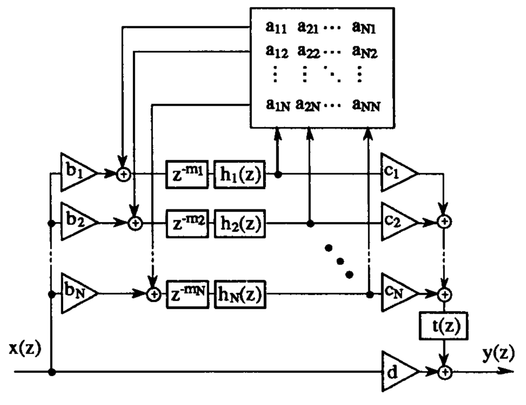
The output of the FDN is given by the following equation, with \(x(t)\) being the input signal and \(q_i(t)\) the output of the \(i^{th}\) delay line [3]:
\[ y(t) = \sum_{i=1}^{N} c_i \cdot q_i(t) + d \cdot x(t) \tag{1}\]
\[ q_j(t+m_j) = \sum_{i=1}^{N} a_{ij} \cdot q_i(t) + b_j \cdot x(t) \qquad (\textrm{for}\ 1 \le j \le N), \tag{2}\]
Which becomes in the z-domain:
\[ y(z) = c^T \cdot q(z) + d \cdot x(z) \tag{3}\] \[ q(z) = D(z) \cdot [A q(z) + b x(z)], \tag{4}\]
where:
\[ q(z) = \begin{bmatrix} q_1(z) \\ q_2(z) \\ \vdots \\ q_N(z) \end{bmatrix} \qquad D(z) = \begin{bmatrix} z^{-m_1} & 0 & \cdots & 0 \\ 0 & z^{-m_1} & \cdots & 0 \\ \vdots & \vdots & \ddots & \vdots \\ 0 & 0 & \cdots & z^{-m_n} \end{bmatrix} \qquad b = \begin{bmatrix} b_1 \\ b_2 \\ \vdots \\ b_N \end{bmatrix} \qquad c = \begin{bmatrix} c_1 \\ c_2 \\ \vdots \\ c_N \end{bmatrix} \qquad A = \begin{bmatrix} a_{11} & a_{12} & \cdots & a_{1N} \\ a_{21} & a_{22} & \cdots & a_{2N} \\ \vdots & \vdots & \ddots & \vdots \\ a_{N1} & a_{N2} & \cdots & a_{NN} \end{bmatrix} \]
The transfer function of the FDN is then given by:
\[ H(z) = c^T \cdot \left[ D(z^-1) - A \right]^{-1} \cdot b + d \tag{5}\]
The \((\cdot)^T\) operator is the transpose operation, the matrix \(D(z^{-1})\) is the diagonal delay matrix, \(A\) is the feedback matrix, \(b\) is the input gain vector, \(c\) is the output gain vector and \(d\) is the direct path gain.
1.1.1 Feedback Matrix
The feedback matrix, sometimes called the mixing matrix, is a \(N\times N\) matrix that defines how the signal is scattered inside the feedback loop. Ignoring the attenuation filters for a moment, it is often desirable for the FDN to be lossless, which happens when the poles of the system all lie on the unit circle. This can be achieved with the use of a unitary feedback matrix [4], [5]. A matrix is said to be unitary if it fulfills the condition:
\[ AA^H=I, \]
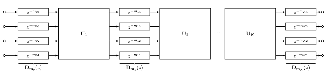
where \((\cdot)^H\) denotes the Hermitian transpose and \(I\) is the identity matrix. Common types of unitary matrices include the Hadamard matrix and the Householder matrix. More complex types of matrix have been proposed in recent years with the goal of improving the echo density of the FDN output. Called filter feedback matrix (FFMs) [6], these are matrices where each entry is a finite impulse response (FIR) filter. These FFMs can be implemented efficiently in a cascaded form, where \(K\) feedback matrices are separated by a bank of delay lines, as shown in Figure 2.
1.1.2 Attenuation Filters
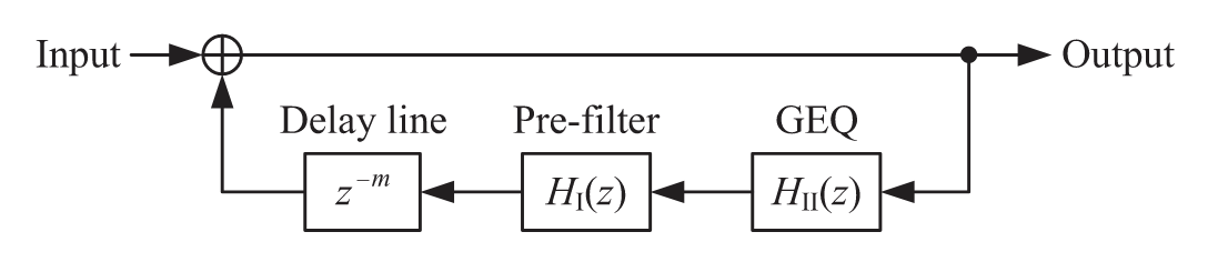
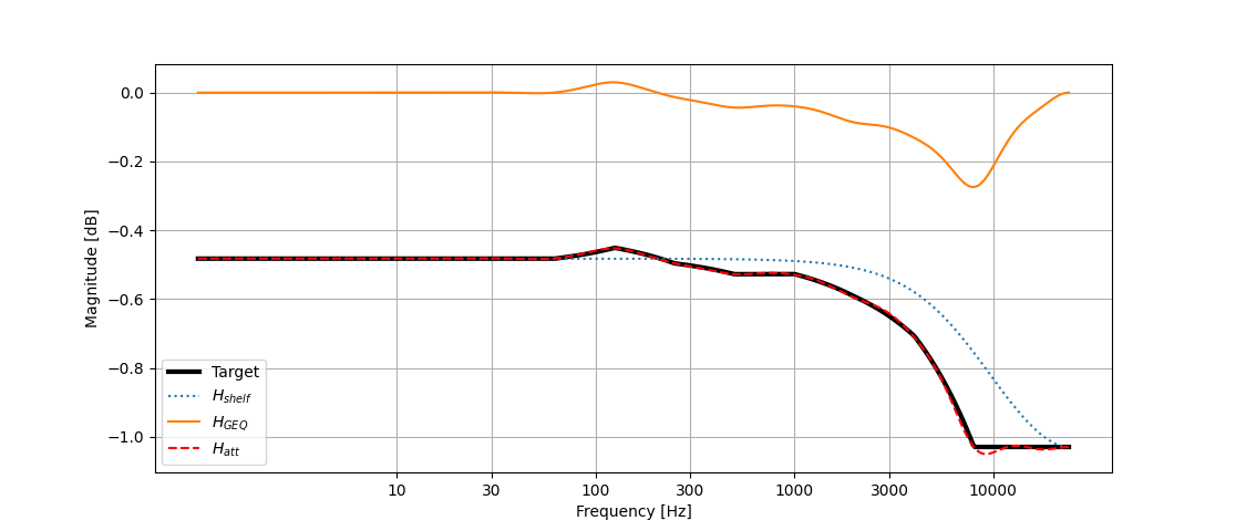
Adding attenuation filters inside the feedback loop allows for control of the frequency-dependant decay time of the FDN. Various strategies have been proposed in the literature to design the filters. One of the first proposed methods involved the use of a one-pole lowpass filter[2] where the pole of the filter depends on the desired reverberation time (\(T_{60}\)) at \(dc\) (0Hz) and the Nyquist frequency and further scaled by the delay length of the preceding delay line. More recently, the use of graphic equalizers (GEQ) has been increasingly popular as low-order filters are not accurate enough to model the decay characteristics of real rooms [7]. Välimäki et al. [7] proposed a two-stage approach to design the attenuation filter where a low-order low-shelf filter is used to approximate the target magnitude response at the \(dc\) and Nyquist frequencies, followed by a higher-order GEQ that can be used to approximate the desired attenuation in multiple frequency bands. The use of the pre-filter eases the design of the GEQ which can become inaccurate if the gain’s variation between bands is greater than 12dB [7].
For this project, an octave band GEQ composed of 10 cascaded biquad filters was used.
1.1.3 Tonal Correction Filter
A tonal correction filter is added to the output of the FDN to shape the initial energy of the impulse response. Jot [3] explains that the use of attenuation filters introduces a dependence between the reverberation time and the frequency response of the FDN. The tonal correction filter is then used to correct the frequency response of the FDN to match the desired target, which in our case would be a real room impulse response. A common method to obtain the gains of the filter is to look at the initial amplitude of each band of the energy decay curves.
2 Room Impulse Response Analysis
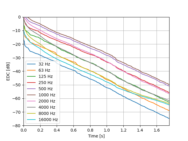
In order to accurately design the attenuation filters and the tonal correction filter, we will need to analyze the target room impulse response (RIR) to extract the desired reverberation time (\(T_{60}\)) at each frequency band. This usually involves looking at the energy decay curves (EDC) of the RIR.
The EDC was first introduced by Schroeder [8] and is defined as the reverse integral of the squared impulse response \(h(t)\):
\[ EDC(t) = \int_{t}^{+\infty} h^2(\tau) d\tau \]
The impulse response is first filtered through an octave band filter bank to obtain the energy decay curves at each frequency band. The EDCs are then scaled to a dB scale to obtain the reverberation time. Depending on the level of static noise present in the RIR, it might be more accurate to compute the \(T_{60}\) using the T15 [9]:
\[ T_{60} = 4 \cdot T_{15} \]
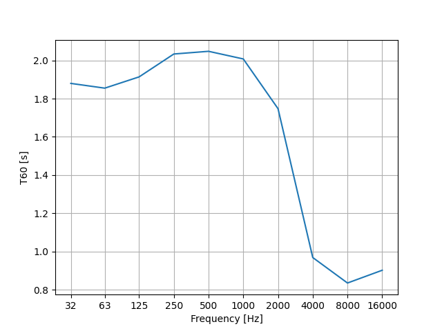
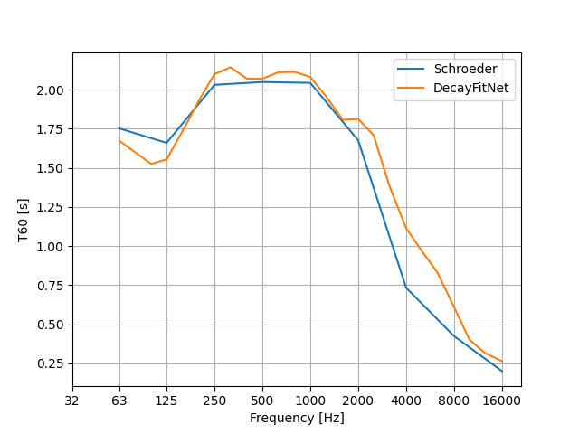
A downside of this method is that the resulting \(T_{60}\) can be greatly affected by the choice of the filter bank used to filter the impulse response [10], [11].
Götz et al. [12] proposed a neural-network-based method for estimating EDCs, called DecayFitNet. This method should be less sensitive to the presence of static noise in the RIR and was the one used for this project.
3 Automatic Optimization
Given the difficulty of choosing the parameters of the FDN manually to obtain satisfactory results, techniques have been proposed to automatically optimize the parameters of the FDN, often with the goal of matching a target RIR.
In [13], Chemistruck et al. used a genetic algorithm (GA) to find the feedback matrix coefficients as well as the cutoff frequencies to the attenuation filters. The FDN architecture used in the experiment was a 4-channel FDN with second-order lowpass filters as attenuation filters. With only 4 channels, the FDN will have difficulties building a realistic echo density, and as such the authors added a diffusion stage to the output of the FDN. The diffusion stage is composed of \(N\) parallel delay lines of length \(\{ D, \frac{D}{2}, \frac{D}{4}, \ldots, \frac{D}{N} \}\), with \(D\) being less than 300 samples. To evaluate the fitness of the FDN, the amplitude envelope of the FDN output was compared to the amplitude envelope of the target RIR. The difference between each sample was summed up and the FDN with the lowest error was selected. Results of listening tests showed the GA reverb output was consistently rated lower than the output generated through convolution with the target RIR.
In [14], Coggin and Pirkle also used GA to optimize the parameters of an FDN. Changes from the previous work include the use of an FIR filter at the input of the FDN to model the early reflections of the target RIR. The coefficients of the FIR filters were obtained by taking the first 80ms of the target RIR. The Hadamard matrix was used as the feedback matrix this time and stayed constant during the optimization. A 16-channel FDN was used. The parameters optimized by the GA were the delay lengths \(m\), the input gains \(b\) and the output gains \(c\). Input and output gains were limited to a range of \([-1,1]\) and delay lengths were constrained to be integer values less than 100ms. Attenuation and tone correction filters were designed based on the \(T_{60}\) of the target RIR. Sixth-order filters were used for the attenuation filters and a 4096-tap FIR filter was used for the tonal correction filter. The fitness function was once again based on the amplitude envelope, but this time the maximum absolute value of the difference between the two amplitude envelopes was used. Listening tests devised to measure the perceptibility of differences between the GA reverb and the convolution reverb showed that the GA reverb was still not able to convincingly match the target RIR.
In [9], Ibnyaha and Reiss introduced a multi-stage approach to optimize the parameters of an FDN. In the first stage, the target impulse response was analyzed using the Schroeder EDC [8] to obtain the \(T_{60}\) at various frequency bands as well as the initial energy of the RIR. This information was used to design the attenuation filters and the tonal correction filter using the graphic equalizer developed by Valimaki et al. in [15]. GA was then used to optimize the value of the delay lengths \(m\), the input gains \(b\), the output gains \(c\) and the direct gain \(d\). Gains were constrained to values between \([-1,1]\) and delay lengths were constrained to be integer values between 2 and 250ms. For the feedback matrix, randomly generated orthogonal matrices were used in a 16-channel FDN configuration. To better match the early reflection and echo density build-up of the target RIR, an FIR filter was used at the input of the FDN. The FIR filter was designed by truncating the RIR at \(t=EDT\), where \(EDT\) refers to the early decay time. The fitness function used was:
\[ C(M_{tar},M_{gen}) = \frac{1}{KN} \sum_{i=1}^{K} \sum_{j=1}^{N} |M_{tar}(i,j) - M_{gen}(i,j)|, \]
where \(K\) is the number of Mel-frequency cepstral coefficients (MFCC), \(N\) is the number of bins, and \(M_{tar}\) and \(M_{gen}\) are the target and generated impulse response MFCCs.
In [16], Santos et al. proposed a differentiable FDN architecture that allows optimization of the parameters of the FDN. The main goal of the optimization process is to minimize the coloration of a lossless FDN. The frequency-sampling method is used to approximate the FDN as a finite-impulse-response (FIR) filter by evaluating the transfer function Equation 5 at \(M\) frequencies. The input gains \(b\), output gains \(c\), and matrix coefficients \(W\) are optimized while the delay lengths \(m\) are fixed. To ensure that the matrix is unitary, the matrix coefficients \(W\) are mapped using the equation: \[ U = e^{W_{Tr} - W_{Tr}^\intercal}, \]
where \(W_{Tr}\) is the upper triangular part of the matrix \(W\) and the operator \((\cdot)^\intercal\) is the transpose operation [16]. Two cost functions were used for the colorless optimization. The first cost function \(L_{spectral}\) minimizes the mean-squared error between the magnitude response of the FDN and a theoretical flat magnitude response. The second cost function, \(L_{temporal}\), is there to penalize sparseness in the coefficients of the feedback matrix as it was found that using \(L_{spectral}\) alone would often cause the feedback matrix to converge towards a diagonal matrix [16]. Analysis of the modal distribution of the output IR as well as listening tests showed that their method was able to reduce coloration in the FDN output. Audio examples are available online.
In [17], Santos et al. used their differentiable FDN in an analysis-synthesis framework to match a target RIR. Once a colorless FDN was obtained using the previously described method, DecayFitNet [12] was used to estimate the \(T_{60}\) of the target RIR and the two-stage approach from [7] was used to design the attenuation filters. The tonal correction filter was designed using the same method but with the pre-filter omitted. Once again, an FIR filter was used to model the early reflections of the target RIR. The FIR filter was designed using the first 2 ms of the target RIR. The amplitude of the FDN output was then further adjusted to match the root mean square of the target RIR. To help with echo density, the unitary matrix used in [16] was replaced with a scattering feedback matrix [6] with four stages where each stage is a different optimized Householder matrix. The transposed configuration (see Figure 7) of the FDN was also used, with the claim that it accelerates the echo build-up [17]. Audio examples are available online.
![]()
4 Implementation - MatchReverb
In [9], Ibnyahya and Reiss implemented their system in MATLAB using the FDN Toolbox [18]. While the FDN toolbox is an indispensable tool for the analysis and synthesis of FDNs, it can also be slow, which is a notable drawback when using an optimization algorithm such as GA as it will restrict the number of solutions that can be explored in a given amount of time. For this reason, a custom FDN implementation was developed in C++. A Python binding was also created to allow the FDN to be used in a Python environment to take advantage of the existing optimization libraries, such as PyGAD. The C++ implementation shows up to a 100x speedup compared to the FDN Toolbox. Another advantage of the C++ implementation is that it allows the use of the FDN in real-time scenarios such as gaming or virtual-reality applications.
4.1 Results
The MATLAB implementation of [9] (MatchReverb) was available online and was used to generate the following RIRs. The genetic optimization was performed over 5 generations with a population of 50 individuals per generation and took 23 minutes to optimze 3 FDNs. The ‘Hybrid’ column was generated using the method described earlier with some modification, while the ‘FDN Only’ column uses the same method, but without the early reflection FIR filter. The target RIRs were taken from the MIT RIR survey[19] and can be found online. Three rooms were chosen for the analysis-synthesis: h001_bedroom, h025_diningroom, and h042_hallway, with average reverberation times of 0.30, 0.94 and 2.02 seconds respectively[17]. The optimization time for the three rooms was around 10 minutes. Some of the modifications found in the source code, which were not in the original paper, include a modification to the fitness function that now takes into account the mean error between the target RIR EDC and the synthesized ones, as well as a bug in the scripts that causes the output gains of the FDN to be set to 1. Another interesting aspect of the implementation is that, while the paper claims the tone correction filter is designed in the analysis stage (ie. before the optimization), the implementation actually first generates an impulse response without any tone filter and then the filter is designed using the energy difference between the initial spectrum of the optimized FDN and the initial spectrum of the target RIR. Furthermore, the paper claims to use the MFCCs of the impulse responses to compute the fitness function, but the implementation actually uses the mel spectrogram of the impulse responses.
While the results of the hybrid FDN sound quite close to the reference RIR, the poor results of the FDN-only version might suggest that the early reflection FIR is doing most of the heavy lifting. The ‘Replica’ column was generated using my own reimplementation of the hybrid FDN. My version of the genetic algorithm was performed over 40 generations with a population of 50 individual and took 11 minutes to optimize the 3 FDNs. The higher generation number did not translate into much better results, as it was found that the FDNs tended to converge towards a local minimum in the first 10 generations.
4.1.1 Impulse responses
Bedroom
Dinningroom
Hallway
4.1.2 Audio Examples - Percussion
Bedroom
Dining Room
Hallway
4.1.3 Audio Examples - Drums
Bedroom
Dining Room
Hallway
4.2 Error visualization
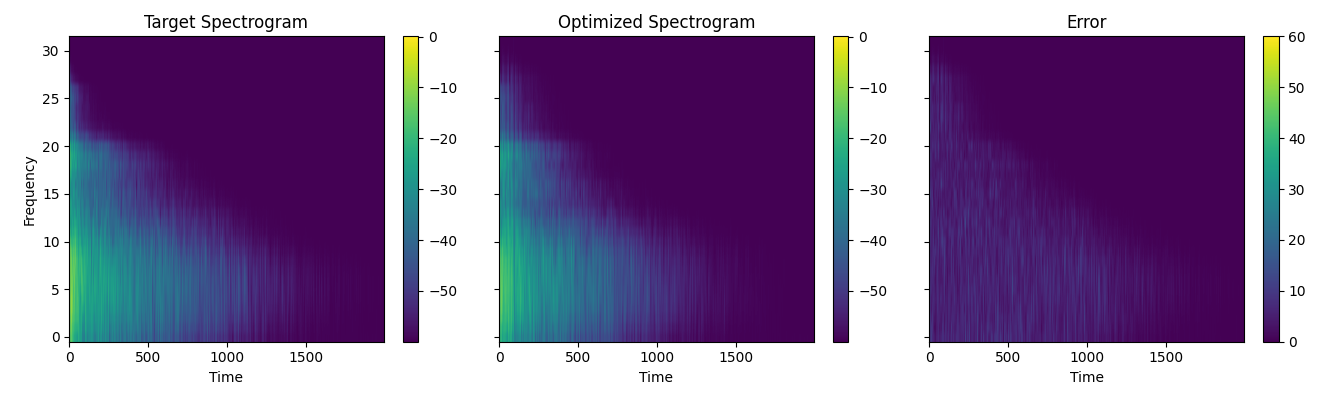
Figure 8 shows the mel spectrogram of the target RIR (left), the FDN output (middle), and the error between the two (right). The error is the absolute difference between the two spectrograms, with a mean error of ~2dB. Even though the error between the two spectrograms is small, the FDN output still sounds noticeably different from the target RIR. This suggests that a fitness function solely based on the spectrogram is not sufficient to accurately match the target RIR using GA.
5 Implementation - RIR2FDN
In [16], [17], [20], Santos et al. implemented the differentiable FDN in the frequency domain using the frequency sampling method. The optimization is implemented in PyTorch and uses the Adam optimizer to optimize a colorless FDN. Once the parameters are optimized, the FDN Toolbox [18] is used to render the final impulse response. The code is available online, as well as audio examples. The implementation uses 1/3-octave band filters for the attenuation and tone correction filters.
I reimplemented the analysis-synthesis framework using my own FDN implementation. The PyTorch optimization was replaced with a genetic algorithm as one of the goals of this experiment is to see if the colorless optimization can be done successfully on a real-time FDN implementation, bypassing the need to build a differentiable proxy as is often done in the literature[21], [22]. The 1/3 octave band filters used in the original implementation were replaced by octave band filters to keep CPU usage low and to see how lower-order filters would affect the results. Audio examples of the optimized FDN, where the scattering matrix was replaced by a simple Householder matrix, are included to better demonstrate the effect of the scattering matrix.
5.1 Result
5.1.1 Impulse responses
Bedroom
Dining Room
Hallway
5.1.2 Audio Examples - Percussion
Bedroom
Dining Room
Hallway
5.1.3 Audio Examples - Drums
Bedroom
Dining Room
Hallway
5.2 Error visualization
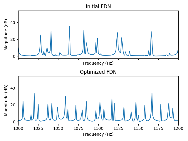
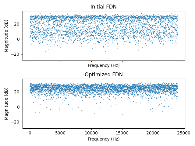
Figure 9 shows the magnitude response of the FDN before and after optimization. The optimized FDN shows a magnitude response with a greater number of peaks and a lower standard deviation. Another useful visualization can be achieved by plotting only the peaks of the full magnitude response. It shows that the distribution of the peaks is much narrower after optimization, which should result in less coloration in the resulting impulse response [23].
6 Conclusion
In this work, we looked into the automatic optimization of feedback delay networks using a genetic algorithm. A real-time FDN implementation was developed in C++ and used within a Python environment to take advantage of the existing optimization libraries. A reimplementation of the methodologies described in [9] and [16], [17] was performed using this new FDN implementation to demonstrate that similar results could be achieved. A potential next step would be to integrate the real-time FDN implementation as a layer of a deep neural network to allow for end-to-end training of the FDN parameters, similar to what was done in [24].
7 Apendix
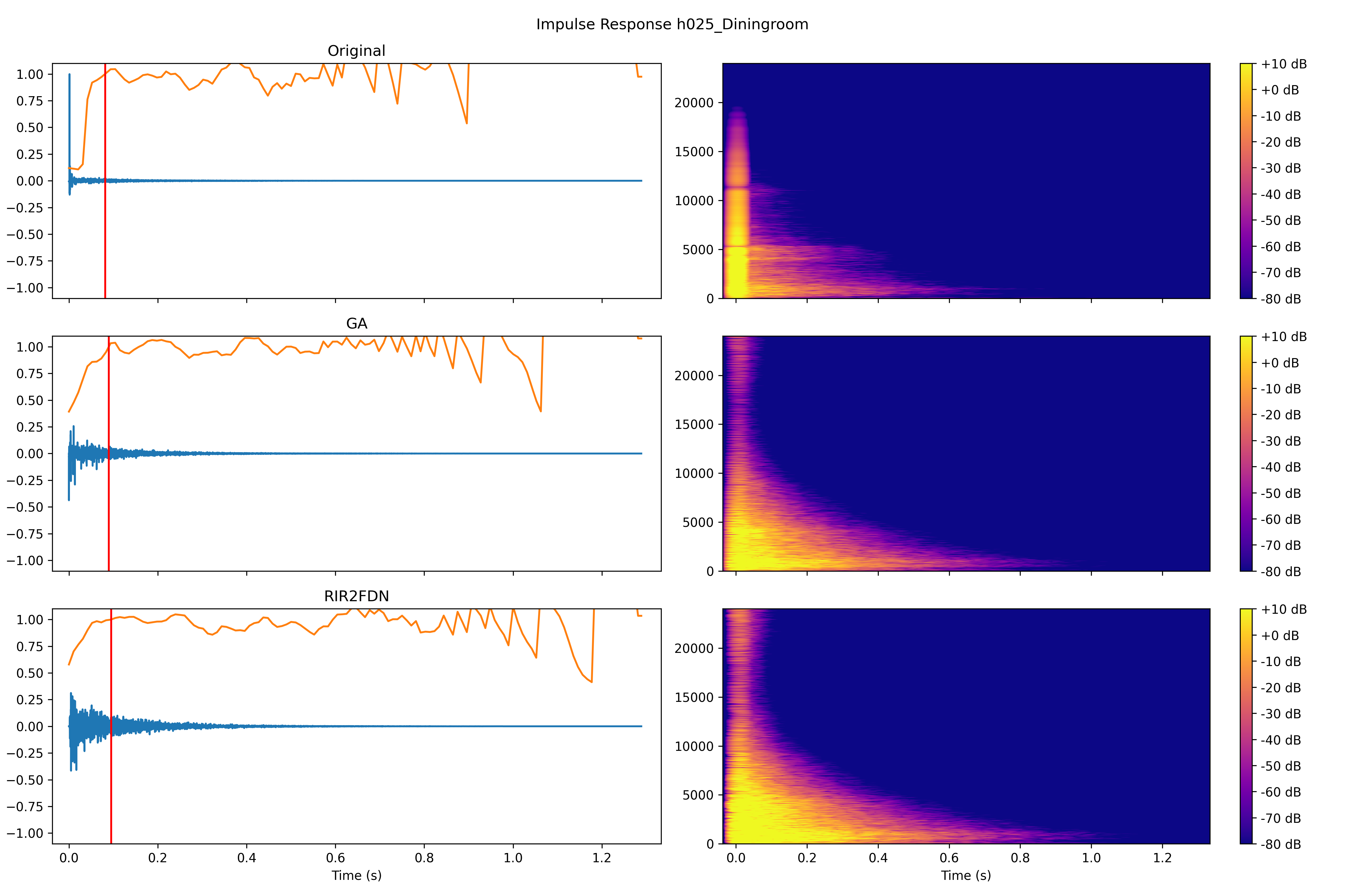
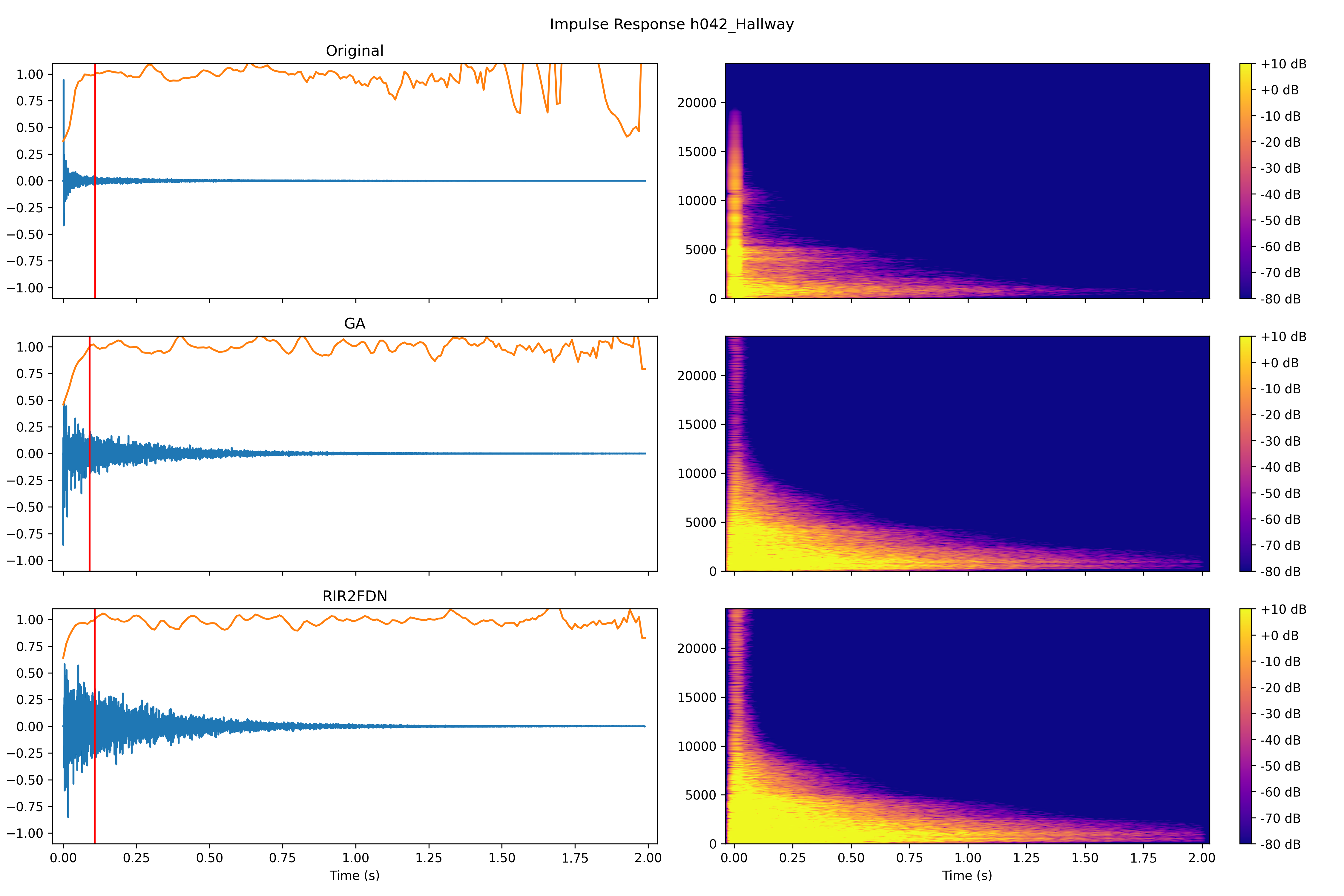
7.1 Spectrograms of synthesized impulse responses
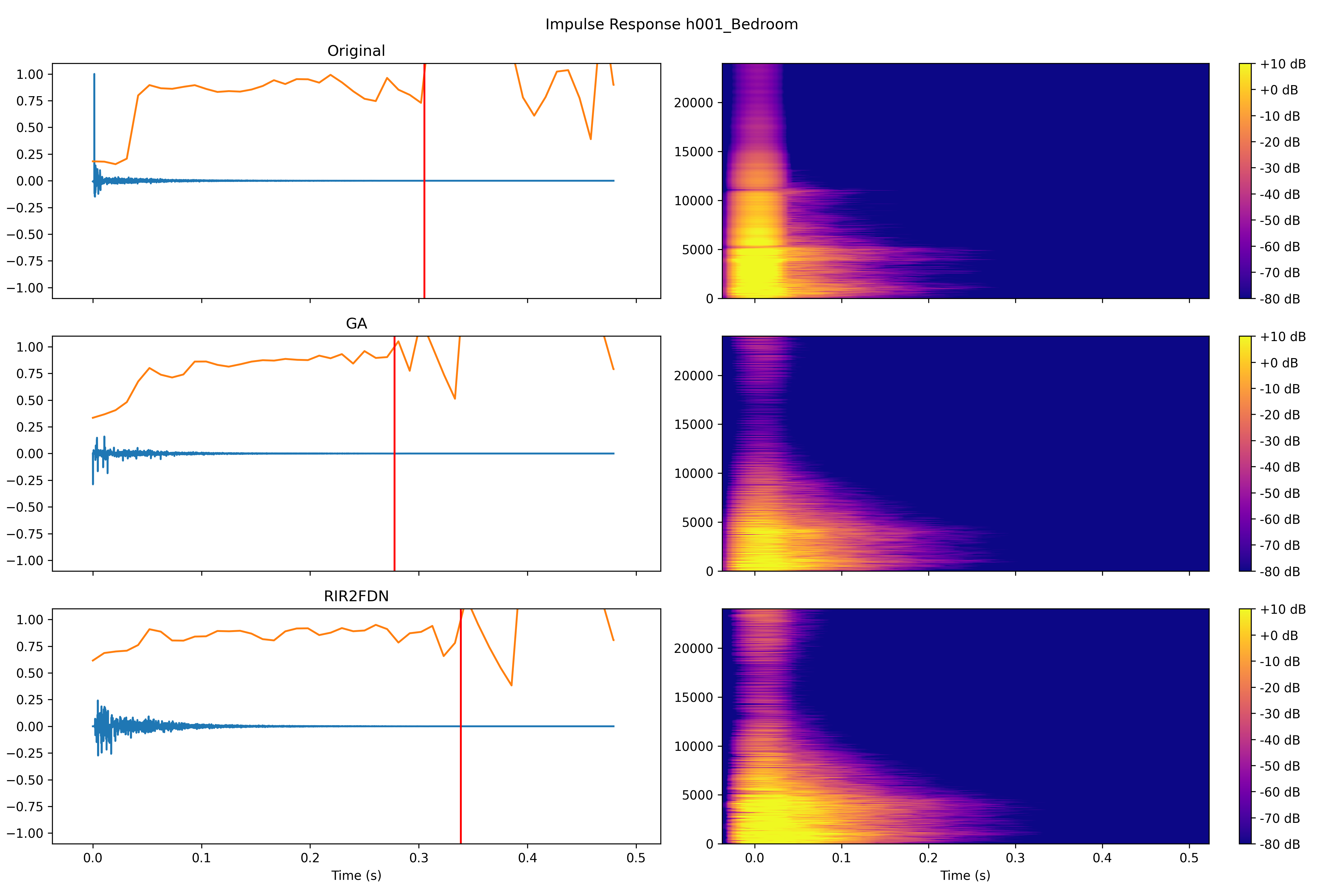
Impulse responses and spectrograms of the target RIR, the synthesized RIR using GA and the synthesized RIR using RIR2FDN. The orange line indicates the echo density profile as proposed by [25]. The red line indicates the time at which the echo density profile reaches a value of 1.
7.2 FDN performance
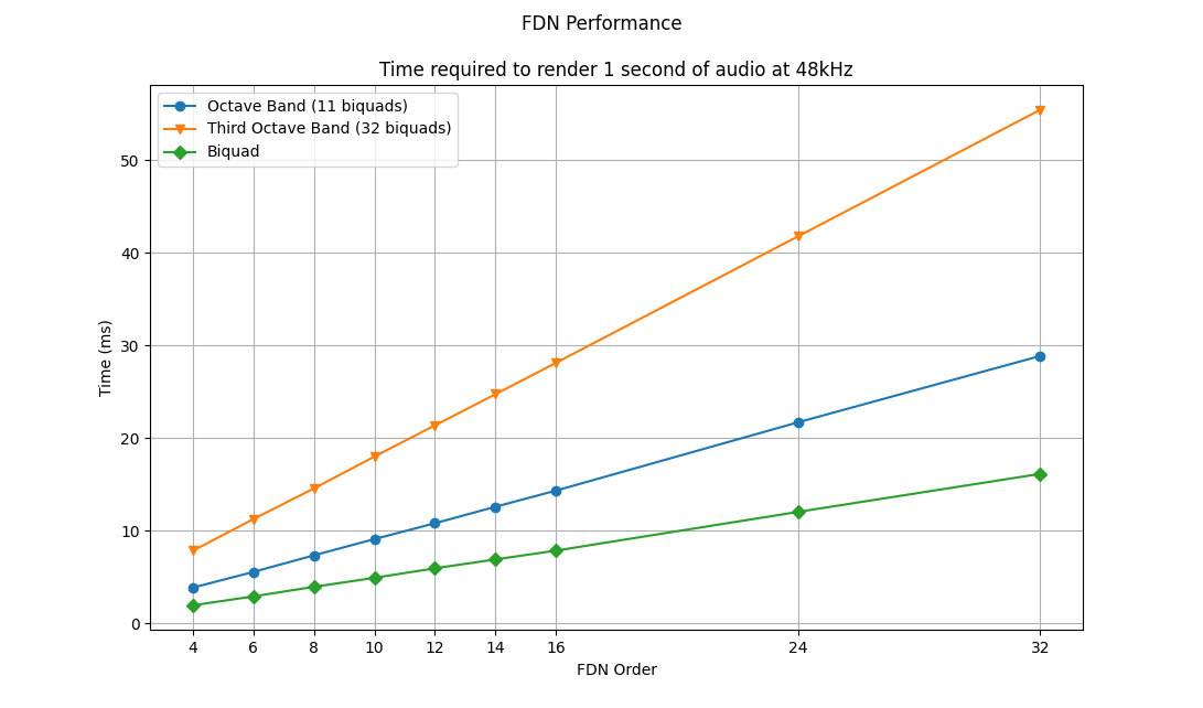
Benchmarks of various FDN configurations. The only difference between the configurations is the number of cascaded biquads used in the attenuation and tone correction filters. A Householder matrix was used as the feedback matrix.
- Blue: 11 cascaded biquads (i.e. octave band filters)
- Orange: 32 cascaded biquads (i.e. 1/3-octave band filters)
- Green: 1 biquad
The benchmarks were performed on a 2024 MacBook Air M3 using the microbenchmarking library nanobench and measured the time taken to render 1 second of audio at 48kHz.