This post is a work in progress. The goal is to provide a comprehensive overview of the performance of feedback delay networks (FDNs) and convolution reverb implementations in the context of room impulse response synthesis.
When comparing feedback delay networks (FDNs) and convolution reverb, FDNs are often said to offer several advantages [1, 2, 3, 4, 5], including :
- Lower CPU usage
- Lower memory usage
- Easier to tune
While it will be difficult to argue against the last two points, the first one should be easily measurable. While FDNs can be used to create a wide variety of reverberation effects, this post will focus on the usage of FDNs as a way to synthesize the acoustic properties of a real room.
Existing benchmarks
DAFx 2020
The first performance measurement of FDNs I could find is from a 2020 DAFx paper by Prawda et al.[6]. The authors built a FDN reverberator based on the state of the art at the time, which includes octave-band attenuation IIR filters and omits the tonal correction filter. The implementation supports block processing, and as such, no vectorized instructions are used.
FDN structure from Prawda et al. [6].
Results from the paper are shown in the table below.
| FDN Order | CPU usage (%) |
|---|---|
| 4 | 5.4 |
| 8 | 7.9 |
| 16 | 13.3 |
| 32 | 30.4 |
| 64 | 92.5 |
The measurements were done on an Intel MacBook Pro using Xcode’s time profiler. It is unclear what exactly was measured, and I suspect a non-negligible amount of CPU time was used by the JUCE framework. Since the code is available on GitHub, I was able to build the project locally and run my own benchmarks by isolating the FDN code from the JUCE framework. The following were the results of my measurements on a MacBook Air M3. The Time (ms) column shows the time it took to process 1 block of 128 samples. The CPU usage (%) column shows how much of the time allocated for one block of audio processing was used by the FDN (ie, at a sample rate of 48000Hz, each audio block has to be computed in less than 2667 \(\mu s\)).
| FDN Order | Time (\(\mu s\)) | CPU usage (%) |
|---|---|---|
| 4 | 21.57 | 0.80 |
| 8 | 44.61 | 1.67 |
| 16 | 113.72 | 4.26 |
| 32 | 324.19 | 12.16 |
| 64 | 850.94 | 31.91 |
Steam audio
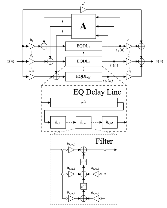
The other benchmark I could find is from the Steam Audio SDK. Steam Audio is an audio solution for game developers that includes, among other things, an FDN reverberator. The open-source code also includes a benchmark for the FDN that I was able to run on my system. As far as I can tell, the FDN implementation is made of 16 channels with attenuation filters composed of 3 cascaded biquad filters. Outside of the feedback loop, 4 allpass filters are cascaded at the output of the FDN (\(A_1(z)\), \(A_2(z)\), \(A_3(z)\) and \(A_4(z)\)) and a tonal correction filter is applied at the end (\(T(z)\)). Below is a diagram of the FDN structure implemented by Steam Audio. Vectorized instructions are used when possible to speed up the execution. Again, the “Time (\(\mu s\))” column shows the time it took to process 1 block of 128 samples.

| FDN Order | Time (\(\mu s\)) | CPU usage (%) |
|---|---|---|
| 16 | 6.9772 | 0.2616 |
Custom C++ implementation
I previously implemented a realtime FDN reverberator in C++. Similarly to the Prawda et al. implementation, octave-band cascaded biquad filters are used for the attenuation filters, and a tonal correction filter was added at the end, using the same octave-band filter structure. The vDSP library is used to speed up the execution of the FDN where possible. Eigen is used for the matrix operations. Again, the “Time (\(\mu s\))” column shows the time it took to process 1 block of 128 samples.
| FDN Order | Time (\(\mu s\)) | CPU usage (%) |
|---|---|---|
| 4 | 7.19 | 0.2696 |
| 8 | 13.65 | 0.5119 |
| 16 | 24.96 | 0.9360 |
| 32 | 50.35 | 1.8881 |
| 64 | 100.90 | 3.7838 |
Computational cost breakdown
The table below shows the breakdown of the CPU usage for each of the major components of a 16-channel FDN. The other category includes mostly the additions in the feedback loop and the addition plus scaling of the direct signal with the reverberated signal.
| Component | Time (\(\mu s\)) | (%) |
|---|---|---|
| Attenuation filters | 21.5519 | 79.79 |
| Mixing matrix | 2.1699 | 8.033 |
| Delay bank | 1.328 | 4.916 |
| Tone correction filter | 1.2316 | 4.559 |
| Others | 0.4150 | 1.5364 |
| Input/Output gains | 0.3156 | 1.1684 |
| Total | 27.012 | 100 |
It is clear that the overwhelming majority of the CPU usage is spent by the attenuation filters. It is worth mentioning that while simpler and cheaper filters could be used, the use of octave-band (and sometimes third-octave-band) filters is common in the literature when the goal is to recreate a real room impulse response [1, 2, 7].
Fast convolution
An alternative to FDNs is to use fast convolution algorithms to convolve the input signal with the room impulse response. Partitioned convolution is a common approach used to convolve a signal with a potentially long impulse response. The thesis by Wefer [8] is a good reference for this approach.
I implemented a simple non-uniform partitioned convolution algorithm in C++ based on Wefer’s thesis. The algorithm uses a very simple partitioning scheme defined as follows:
\[ P = \left( \left[B\right]^4, \left[4B\right]^4, \left[8B\right]^4, \left[16B\right]^N \right), \]
where \(B=128\) is the block size and \(N\) increases as needed depending on the size of the FIR. A benchmark of the partitioned convolution algorithm was done by convolving a signal with a FIR filter of length ranging from 10000 taps to 144000 taps (ie, 3s of audio at 48000Hz).
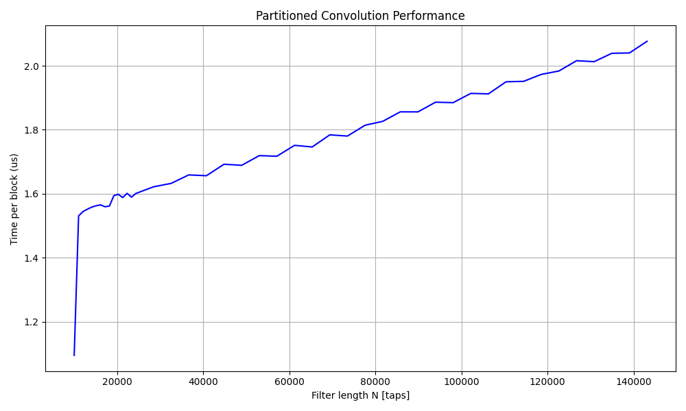
The results of the benchmark show that the partitioned convolution algorithm is almost 3 times faster than the Steam Audio FDN, ~50 times faster than the 16-channel FDN from Prawda et al., and ~10 times faster than my custom C++ implementation when convolving with a 3s FIR filter. It is also worth noting that this was my first attempt at implementing a partitioned convolution algorithm, and there is no doubt that it could be optimized much further based on the more recent work published on the subject.