BowedString Part 2: Bow Table

Now that we have our working waveguide, we need something to excite it. This is done with the help of a bow table. While the linear bow table would be simple to implement, we would need to know the capture or break-away differential velocity value \(v_\Delta^c\) and also how this value responds to varying force values. I could not find a simple way to find these values but luckily, the STK library has a bow table that we can reuse.

Let’s take a look at the bow table as defined in the stk:

\[ BowTable(v_\Delta^+) = \min \left \{(|v_\Delta^+|*Slope + 0.75)^{-4}, 1 \right \} \]

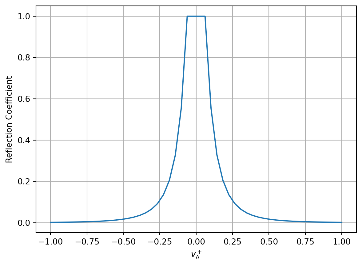
Where \(v_\Delta^+\) is the velocity of the bow minus the velocity of the string going into the bow and \(Slope\) is the parameter that controls the shape of the table and is related to the bow force. While the equation may seem daunting at first, we can easily plot it and immediately recognize a shape similar to the linear bow table as presented by figure 9.54 in Physical Audio Signal Processing by Julius O. Smith.

Code

import numpy as np
import matplotlib.pyplot as plt
from matplotlib.ticker import MultipleLocator

v_delta = np.linspace(-1, 1, 50)
bow_force = 4

output = np.minimum(pow(abs(v_delta) * bow_force + 0.75, -4), 1)

plt.figure(1)
plt.plot(v_delta, output)
plt.xlabel('$v_\Delta^+$')
plt.ylabel('Reflection Coefficient')
plt.grid()

<>:12: SyntaxWarning: invalid escape sequence '\D'
<>:12: SyntaxWarning: invalid escape sequence '\D'
C:\Users\Alex\AppData\Local\Temp\ipykernel_12000\4158656264.py:12: SyntaxWarning: invalid escape sequence '\D'
  plt.xlabel('$v_\Delta^+$')

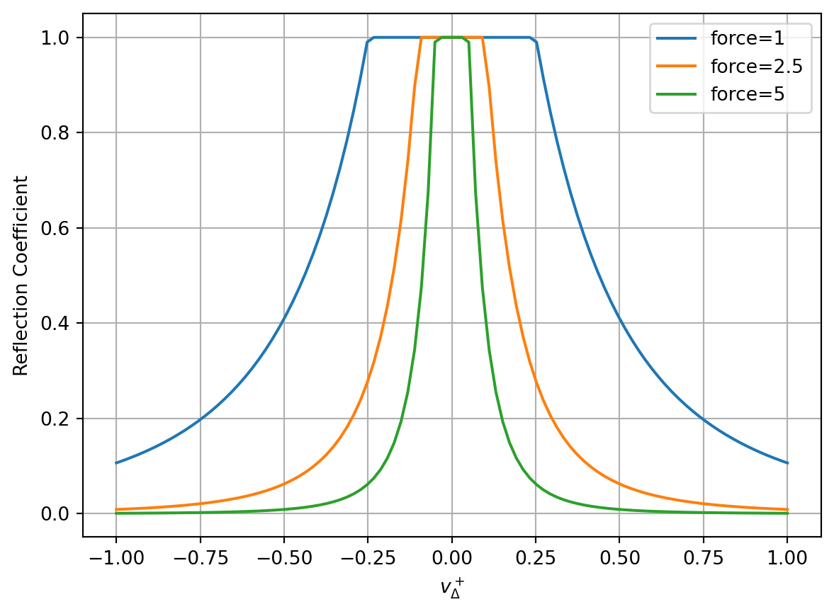
We can now observe how varying the force transforms the bow table.

Code

v_delta = np.linspace(-1, 1, 100)

plt.figure(2)
for f in [1, 2.5, 5]:
    output = np.minimum(pow(abs(v_delta) * f + 0.75, -4), 1)
    plt.plot(v_delta, output, label=f'force={f}')
plt.legend()
plt.xlabel('$v_\\Delta^+$')
plt.ylabel('Reflection Coefficient')
plt.grid()

As \(Slope\) goes up, the region of the table where the reflection coefficient is 1 gets smaller. This plateau represents the moment where the bow and the string are “sticking” together.

We now need to find what is the usable range for \(Slope\). Looking at the STK again, we can see where the slope is set:

bowed.cpp

    bowTable_.setSlope( 5.0 - (4.0 * normalizedValue) );

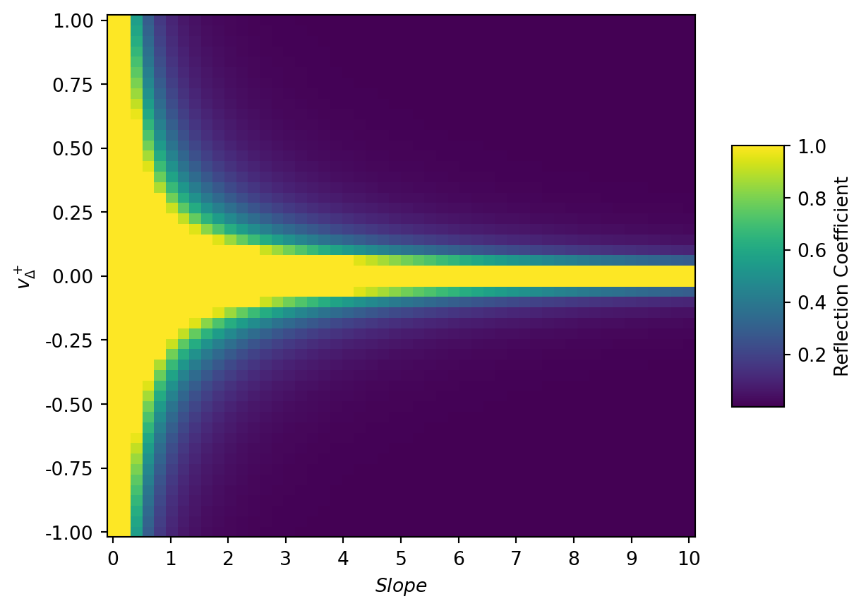
Where normalizedValue is a value between 0 and 1 representing the bow pressure. This effectively restricts the slope value between 1 and 5. In other words, as the bow pressure increases, the ‘sticking’ zone of the bow table gets larger. We can plot the bow table equation again, but this time with varying force values between 0 and 10 to understand why.

Code

v_delta = np.linspace(-1, 1, 50)
f_bow = np.linspace(0, 10, 50)

v_delta, f_bow = np.meshgrid(v_delta, f_bow)
output = np.minimum(pow(abs(v_delta) * f_bow + 0.75, -4), 1)

fig, ax = plt.subplots()
surf = ax.pcolormesh(
    f_bow,
    v_delta,
    output,
    linewidth=0,
    cmap='viridis',)

fig.colorbar(surf, shrink=0.5, aspect=5, label='Reflection Coefficient')

ax.yaxis.set_major_formatter('{x:.02f}')
ax.xaxis.set_major_locator(MultipleLocator(1))
ax.set_xlabel('$Slope$')
ax.set_ylabel('$v_\\Delta^+$')
ax.dist = 10

Looking at the graph, we can immediately see that once the slope gets higher than 5, the reflection coefficient returned by the table stays consistent and there’s limited value for a bow table to support a slope value higher than 5. On the other hand, with a slope value \(<1\), the table becomes almost flat.